Network Training

Once you have created your training images (see Creating Training Images), you can train a detection network. This page walks through each dialog in the training process and explains the settings. The architectures, hyperparameters, and anchor boxes referred to here are described in more detail in Architectures, Hyperparameters & Metrics.

Starting Training

Open the tool. Go to Tools > Network Training > Train Detection Network.
Select the image table(s). DeepAcoustics asks you to select the image table(s) (_Images.mat) for training. You can select more than one, for example to combine image tables made from different datasets, but they must all be in the same folder. It is usually easiest to keep your detections files in one folder, create an image table from them, and save any later image tables in that same folder. In this example, we select the image table created on the previous page.
Add validation image tables (if you have them). DeepAcoustics asks Do you have Validation Image Tables, too?
- Yes: select the validation image table(s) (_ValImages.mat). You will only have these if you set Manually Select Validation Data to Yes when creating the training images. The validation tables must contain the same call types as the training tables.
- No: continue without them. You will have the option to set aside a portion of your training data for validation later on. In this example, we select No.
Choose whether to build on an existing network. DeepAcoustics asks Train from existing network?
- No: train a new network from scratch. Select No. This is the option to use for now.
- Yes and Yes - TensorFlow: build on an existing DeepAcoustics network or a TensorFlow model. These options are still being developed and improved, so we do not recommend them at this time.
Confirm the call types. A Call Types Warning lists the call types the network will be trained on (in this example, 18 Hz, 20 Hz, A, B, and Noise). If you added random noise when creating the training images, Noise appears as one of the call types. Click Yes to proceed.

Call types are fixed once a network is trained

Because of MATLAB limitations, you cannot later add new call types to a network. If you want a network that detects additional call types in the future, you will need to train a new network from scratch with all of the call types included.

Training Settings

A series of dialogs then asks for the training settings. The first prompts you with the architecture you would like to select.

Base network

Choose the base network (architecture) to train from:

Tiny YOLO (pre-trained): the smallest and fastest to train. A good starting point for testing your other settings. This example uses Tiny YOLO.
CSP-DarkNet-53 (pre-trained): the largest and most complex architecture, with an extra detection head.
ResNet-50 (pre-trained): in between the two in size. It always uses an input size of 224 × 224 pixels.
ResNet-50 (blank): a ResNet-50 that has not been pre-trained. This option is still being evaluated.

See Available architectures for a comparison.

Image resolution

For Tiny YOLO and CSP-DarkNet-53, DeepAcoustics asks Would you like to reduce your image resolution b/c your GPU crashed the last time you tried this?

No - I believe in my GPU: keep the image resolution. Choose this if you have a reasonably powerful computer and GPU.
Yes - I want to edit: enter a smaller image size. Use this if training has previously crashed because your computer ran out of GPU memory.

These architectures require an image size that is a multiple of 32, so DeepAcoustics rounds the size automatically (for example, 300-pixel training images are used at 288 pixels). Choosing a size larger than the resolution you used to create the images does not add detail: the effective resolution stays at the resolution of your training images.

Customize or use defaults

DeepAcoustics asks whether you want to Customize your network options or use the Defaults. We recommend Customize in most cases. If you choose Defaults, DeepAcoustics uses 8 anchor boxes (9 for CSP-DarkNet-53), the SGDM solver, a learning rate of 0.01, a mini-batch size of 16, 30 epochs, and no validation data, and skips the rest of the settings below.

Anchor boxes

DeepAcoustics asks Do you already know how many anchor boxes you want to use?

Yes: enter the number of anchor boxes directly.
No: DeepAcoustics calculates the best anchor boxes for every count from 1 to 15 and plots the results so you can choose.

When you select No, here is what DeepAcoustics calculates:

For each number of anchors from 1 to 15, it groups the widths and heights of all the bounding boxes in your training images into that many clusters (using MATLAB’s estimateAnchorBoxes, a clustering method that groups boxes by how much they overlap). The center of each cluster becomes one anchor box shape.
For each count, it calculates the mean IoU: how well, on average, each of your annotated boxes overlaps with its closest-matching anchor shape. A mean IoU of 1 would mean every box matched an anchor exactly.
It plots Number of Anchors (x-axis) against Mean IoU (y-axis).

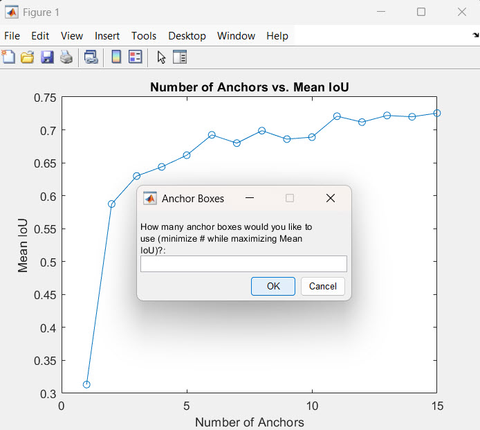
Choose the number where the curve starts to level off (the “elbow”). Beyond that point, adding more anchors improves the fit only slightly while increasing computation. In this example, the curve rises steeply up to about 6 anchors and then flattens, and 6 anchors has also worked well for us in the past, so we enter 6. We also recommend trying a few values and comparing the resulting networks.

If the number you enter does not suit the architecture, DeepAcoustics rounds it up: Tiny YOLO and ResNet-50 need an even number, and CSP-DarkNet-53 needs a multiple of three. See Anchor boxes for how anchor boxes work and how to choose the number.

Solver (optimizer)

The solver, or optimizer, is the algorithm that adjusts the network’s weights during training to reduce the loss (the error between the network’s predictions and your annotations). DeepAcoustics currently offers three:

sgdm (stochastic gradient descent with momentum): after each mini-batch, takes a step in the direction that reduces the loss, using the same step size (learning rate) for every weight. “Momentum” carries over part of the previous steps, which smooths out the path and helps it keep moving in a consistent direction. It is simple and reliable but can need more epochs to converge.
rmsprop (root mean square propagation): adjusts the step size separately for each weight, based on how large that weight’s recent updates have been. Weights with large or erratic updates take smaller steps, and weights with small, steady updates take larger ones. This often makes training more stable. RMSProp has worked well for us, and we typically use it with its default learning rate.
adam (adaptive moment estimation): combines the two ideas above: it uses momentum like SGDM and adjusts each weight’s step size like RMSProp. It often converges quickly and is a common default in deep learning.

Initial learning rate

The learning rate sets how large a step the solver takes each time it updates the weights. The suggested defaults are 0.01 for sgdm and 0.001 for rmsprop and adam. A rate that is too high can make training unstable (the loss jumps around or grows); a rate that is too low makes training very slow. If training runs into problems with your computing resources, try a lower rate. This is a setting worth experimenting with.

Mini-batch size

During training, the training images are shuffled and divided into small groups called mini-batches. The network processes one mini-batch, calculates the average loss across those images, and then updates its weights once. Each of these updates is one iteration, so the number of iterations in one epoch is roughly the number of training images divided by the mini-batch size.

Larger mini-batches give a more stable estimate of which direction to adjust the weights and need fewer updates per epoch, but they use more GPU memory.
Smaller mini-batches use less memory and make more frequent, noisier updates.

The default is 16, because larger architectures such as CSP-DarkNet-53 can run out of memory with bigger mini-batches. Smaller networks such as Tiny YOLO can usually handle larger mini-batches, such as 64 and above.

Maximum number of epochs

An epoch is one complete pass through all of the training images (see Key hyperparameters). The default maximum is 30. More epochs give the network more chances to learn, but training too long can lead to overfitting, where the network memorizes the training images instead of learning patterns that generalize to new data. Watch the training progress window (below) and stop early if the validation loss starts to rise.

Validation data

If you did not provide validation image tables, DeepAcoustics asks Would you like to use a proportion of your training data to validate (recommended to assess overfitting)?

Yes: set aside part of your training images for validation. These images are not used to train the network; instead, the network is checked against them during training to show how well it handles data it has not learned from. This is what lets you spot overfitting.
No: train on all of the images without validation (not recommended).

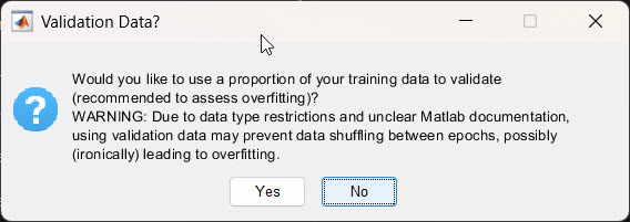
The dialog also warns that, because of MATLAB data type limitations, using validation data may stop the training images from being reshuffled between epochs, which could itself contribute to overfitting.

If you choose Yes, enter the proportion of your non-augmented training images to use for validation, as a decimal (the default is 0.1, or 10%). Augmented duplicates are never selected for validation. Studies have used validation proportions from about 10% up to 25%; we have found that about 0.2 (20%) works well, and that is what this example uses.

How the validation images are chosen

With a multiclass network, DeepAcoustics tries to make sure every call type is represented in the validation set:

It counts how many (non-augmented) training images contain each call type.
It multiplies the count for the rarest call type by your proportion. This becomes the number of validation images for every call type, so each call type gets roughly the same number of validation images.
Starting with the rarest call type, it randomly selects images containing each call type until that call type has its share. Because one image can contain several call types, images selected for one call type also count toward the others.

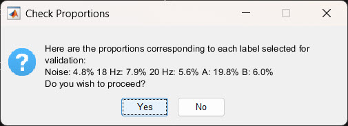
DeepAcoustics then shows a Check Proportions dialog with the percentage of each call type’s images that ended up in the validation set. The rarest call type will be close to the proportion you entered, and more common call types will be lower, because they all receive about the same number of validation images. In this example, with a proportion of 0.2, call type A (the rarest) is at 19.8%, and the more common call types are between 4.8% and 7.9%. Click Yes to proceed (clicking No cancels training).

Monitoring Training

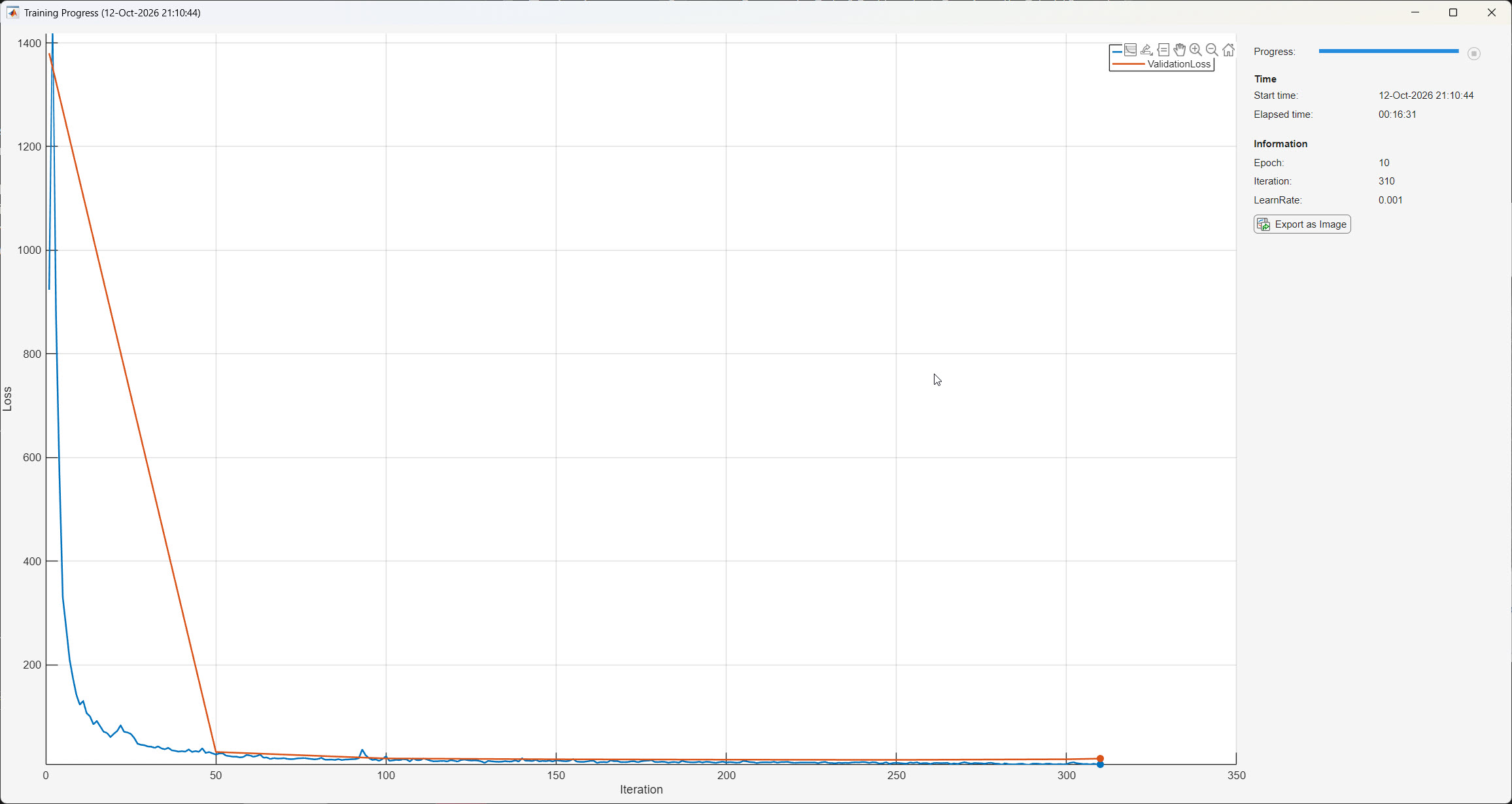
Once the settings are confirmed, training begins and the Training Progress window opens.

TrainingLoss (blue line): the loss on the current mini-batch of training images, plotted at every iteration. It is usually very high at first and then drops quickly as the network starts to learn, before leveling off.
ValidationLoss (orange line): the loss on the validation images. It is calculated only every so often (every 50 iterations by default in MATLAB), so it appears as points joined by straight lines, which can look like a long straight line early in training.
Progress panel (right): shows the progress bar, start time, elapsed time, current epoch, iteration, and learning rate. The Export as Image button saves a picture of the plot.

How to read the curves is explained in Key hyperparameters. In short: if both losses fall together, the network is still learning; if both are low and stable, the fit is good; and if the validation loss starts to rise while the training loss keeps falling, the network is overfitting.

The MATLAB Command Window

While training runs, MATLAB also prints a progress table in the Command Window. It starts by listing the call types (object classes) the network is being trained on, then adds a row every 30 iterations, plus a row each time the validation loss is calculated:

Epoch   Iteration   TimeElapsed   LearnRate   TrainingLoss   ValidationLoss
  1         1        00:00:09       0.001        923.51          1380.1
  1        30        00:01:47       0.001        42.379
  2        50        00:02:51       0.001        26.871          31.749
  ...
  9       250        00:13:20       0.001        10.69           16.467
 10       300        00:15:56       0.001        8.3519          17.686
 10       310        00:16:27       0.001        8.2466          18.928

Epoch: which pass through the training images the network is on.
Iteration: how many weight updates (mini-batches) have been completed so far. In this example, 10 epochs took 310 iterations, or about 31 iterations per epoch.
TimeElapsed: the time since training started (hours:minutes:seconds).
LearnRate: the learning rate in use. It stays at the initial learning rate you entered throughout training.
TrainingLoss: the loss on the current mini-batch of training images.
ValidationLoss: the loss on the validation images. It is only filled in on the rows where it was calculated (every 50 iterations, and at the end of training); it is blank on the other rows. If you did not use validation data, this column does not appear.

When training is complete, MATLAB prints Detector training complete.

This table holds the same information as the Training Progress window, but as exact numbers, which makes it easier to see where the validation loss was lowest. In this example, the training loss keeps falling right to the end (from 923.51 to 8.2466), but the validation loss reaches its lowest value, 16.467, at iteration 250 (epoch 9) and then rises to 17.686 and 18.928. That rise while training loss keeps falling is an early sign of overfitting, and it suggests that about 9 epochs would have been enough for this dataset and these settings.

Early stopping

Early stopping means ending training before the maximum number of epochs, at the point where the network performs best on the validation data. If the validation loss stops improving or starts to rise while the training loss keeps falling, further training is likely to make the network worse at handling new data. To stop early, click the stop button (the round button to the right of the progress bar). The network is kept as it was when you stopped, so stop near the point where the validation loss was lowest. You can also use what you see to choose a smaller number of epochs the next time you train.

Saving the network

Save the trained network

When training finishes (or you stop it), DeepAcoustics opens a Save New Network dialog. You must save the network here, or the training will be lost. The network is saved as a .mat file, but the dialog does not suggest a file name, so give it a clear, descriptive name. For example, include the project or dataset, the architecture, the call types, and a version number, such as OOI_Multiclass_TinyYOLO_6anchors_v1.mat. Because training images, detections, and networks are all .mat files, a clear name makes it much easier to tell your networks apart later.

The network .mat file stores the trained detector together with the training options and the spectrogram settings used to create the training images (window size, overlap, NFFT, frequency limits, sampling rate, and image length), so DeepAcoustics knows how the network’s images were made when you use it to detect calls. Save it in your networks folder so it appears in the Neural Networks list in the main window.