OPTICS Modeling
OPTICS utilizes multi-parameter statistical regression to determine a combination of in-situ variables that best predicts chemical contaminant concentrations with high variance. OPTICS applies is a statistically based method that identifies combinations of multi-collinear predictors (in-situ, high-resolution measurements) that have large covariance with a response (discrete surface water chemical contaminant concentration data from samples that are collected periodically, coincident with in-situ measurements). The technique combines information about the variances of both the predictors and response, while also considering the correlations among them; therefore, providing a tool with reliable predictive power.
Performing Regression Analyses
The “Run regression” button selected from the “Input” tab performs the regression analysis with the set of sensor variables and filters set by the user. Multiple regressions can be run and compared by navigating back to the “Input” tab, modifying the inputs by transforming the data or further filtering and selecting the “Run regression” button again. Each regression analysis is labeled with the date, time and transformation state (e.g., “none,” “log”) appended to the filename. Results from all analyses are listed in the top right section of the “Regression” tab, allowing for each comparison between results. Selecting an analysis run from the “Regression ID” field loads the figures related to that analysis. An analysis run can be deleted by highlighting the name in the “Regression ID” field and hitting the “delete” tab.
Regression Results
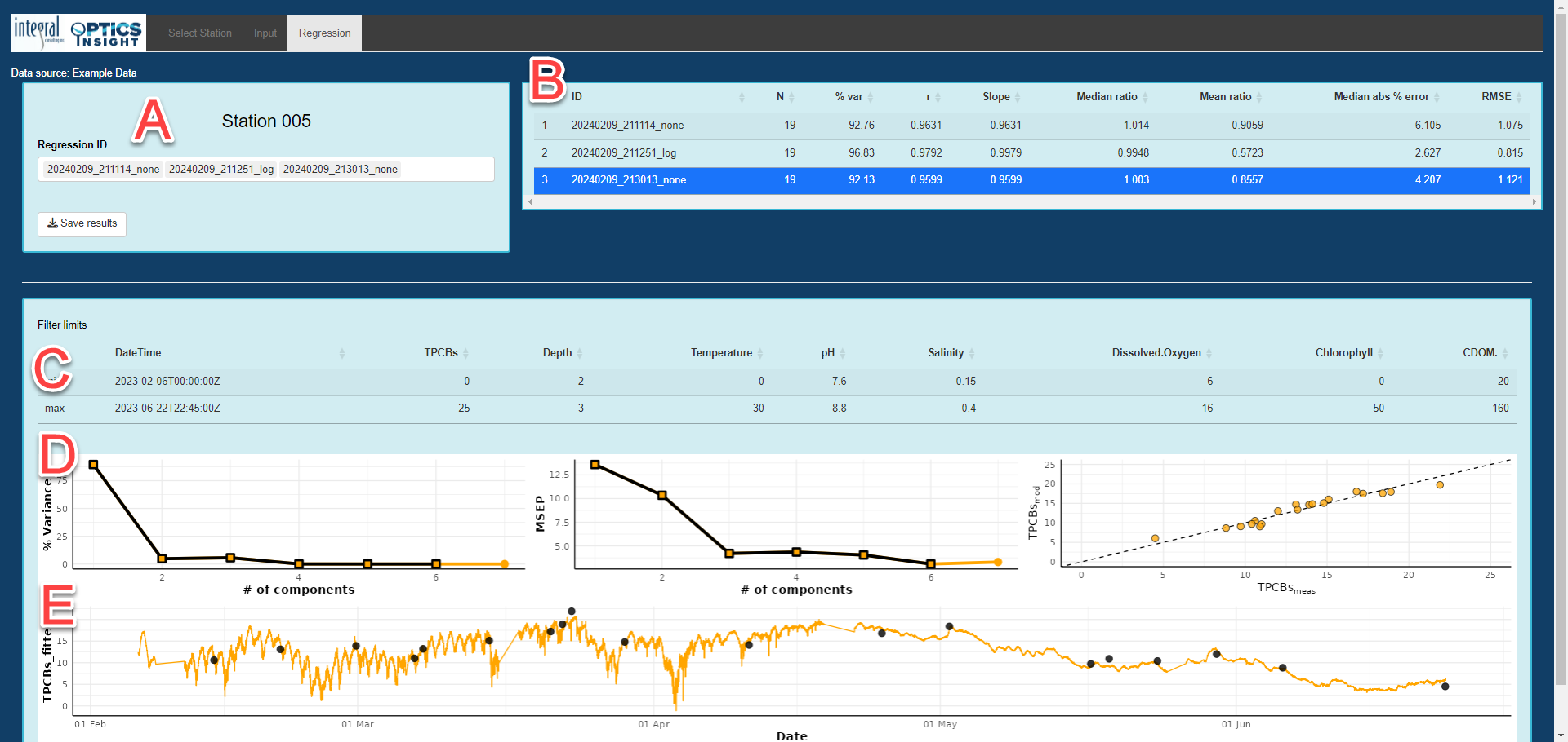
The results from an analysis run are summarized in tabular and graphical format on the “Regression” tab. In the results figure below:
A) List of available regression analyses and “Save results” button to download output from analyses. The date, time and transformation (“none” meaning no transformation) is stored in the filename for each run. The date and time is in GMT, as the processing is done virtually and cannot access your local computer time.
B) Table of OPTICS performance statistical metrics including:
N = Number of samples included in the calculation of statistical metrics.
% var = Percent variance explained, or the proportion to which the OPTICS model accounts for the variation in the data set. A higher percentage of variance explained indicates that the OPTICS model can better predict or capture the variability present in the data set. Conversely, a lower percentage suggests that the model may not adequately capture the complexity or underlying structure of the data.
r = Correlation coefficient (Pearson’s R), a result from linear regression that is a measure of the linear correlation between two variables (i.e., how well data1 are correlated to data2), assuming that both data1 and data2 may contain some error. The values of r that indicate the best model fit are typically close to 1 or -1, suggesting a strong positive or negative linear relationship respectively, between the two variables.
Slope = Model II Slope, a result from linear regression that represents the rate of co-variance in data1 and data2. Model II regressions assume that both data1 and data2 may contain some error. A value of 1.0 indicates no bias in the best-fit regression line signifying optimal model fit; however, it is important to note that the Slope is not a measure of bias in the model or discrete sample data. Therefore, while a Slope of 1.0 suggests ideal alignment, other metrics should also be considered to comprehensively evaluate model performance.
Median Ratio = Median value of the ratio of data1 to data2; i.e., median of (data1 / data2), a measure of overall over- or under-prediction of a model. A Bias value of 1.0 indicates no bias, with values deviating from 1.0 indicating over- or underestimation of the tendencies of the model. Bias is unitless.
Median abs % error = median value of the absolute percent difference between data1 and data2; i.e., Median abs % error = 100 * |data1 – data2| / data2. Median abs % error is a measure of random error. A mean abs % error value of zero indicates no random error, suggesting better model performance.
RMSE = Root mean square error, a measure of the differences between data1 and data2. RMSE =
The RMSE aggregates the magnitudes of the errors in model predictions in a single measure of predictive power and is a good measure of model accuracy. RMSE is in the same units as the input data. Lower values of RMSE indicate better model performance, with RMSE = 0 indicating optimal model performance.
C) Filter setting associated with the regression analysis as determined from the “Input” tab when data were filtered.
D) The left-most figure shows the proportion to which the OPTICS model accounts for variation in the data set (i.e., percent variance) as a function of number of model components. The middle figure shows the mean squared error of model predictions (MSEP) as a function of number of model components. In the left and middle figures, the largest number represented by square symbols is the number of components at which MSEP is minimized and is the number of components used to generate OPTICS model results (shown in the right-hand plot and time series figure below). The right-most figure is a modeled versus measured scatterplot and the dashed line is the 1:1 line.
E) OPTICS model-predicted time series in orange and analytical sample data in black dots for comparison.
Saving Results
Results from multiple regression analyses can be output simultaneously using the “Save results” button on the “Regression” tab. The results consist of: 1) and html file that contains the analysis table and all figures organized by analysis, 2) a .csv filter file documenting all settings used for data query and filtering per analysis, 3) compiled model results into a single .csv file and 4) predicted values by analysis in .csv files. All results (including all regressions that were generated) are saved locally to a folder designated by the user, and are labeled with “OPTICS Insight Summary…” along with the date and time you generated the results.
NOTE: upon completing the analysis, save all outputs immediately as OPTICS Insight disconnects after an extended pause (> 5 minutes) from interacting with the tool.
Returning to the Station Selection Window
Upon completion of OPTICS modeling for a given station, results should be saved prior to returning to the station selection window. All results are cleared after navigating back to the “Select Station” tab, and a warning will remind users that data analyses are not saved after leaving.
Best Practices
The OPTICS modeling analytical process expects the user to be familiar with the statistical approach used in this tool, and can effectively interpret data. We encourage users to evaluate regression results to determine what is most appropriate for their specific dataset. Study design and data analysis best practices include:
Performing a power analysis before data collection is recommended to determine the minimum number of samples required for OPTICS modeling. Samples should cover the widest range of variability possible, which is dependent on the dynamics of the study area. For a tidal system, it is appropriate to sample during spring and neap tide at peak and slack tidal velocities. For systems that are anticipated to change with high flow (e.g., as a result of storms), it is appropriate to sample during or just following storms as possible.
Opting to transform data requires statistical knowledge of when to implement this process. Generally, if the laboratory data are not normally distributed, a transformation is appropriate. Additionally, exploring modeled versus measured results without a transformation may lead a user to transform the data if there is “spray” in the data or curvature in the regression.